
Forget everything you know about playing with toys. This isn’t about circling a track mindlessly. We’re putting on our engineer hats and diving into the physics that makes locomotion possible.
Think of it as a crash course in kinematics, but with more whistles and less homework dread. We’re channeling the same analytical spirit as the visionaries behind futuristic concepts like vacuum tube transportation. They blend physics with big dreams.
Our mission? To get hands-on with the fundamental equation of motion: speed = distance/time. This simple relationship governs everything from a toy chugging along a table to a bullet train crossing a continent.
Through this project, you’ll learn to measure, calculate, and analyze motion like a true STEM investigator. You’ll see how a basic setup can teach unit conversion, data collection, and the scientific method. It’s math and physics in action, debunking the myth that equations only live in textbooks.
Ready to begin? Let’s start by understanding how to calculate the speed of toy and apply those principles to our own miniature world.
Building a Straight Test Track with Markers
Forget the scenic loops and complex switches. We’re making the I-95 of model railways: a long, straight track. It’s for data, not daydreams. As our source says, “Building a stable and functional track is the first step in any train experiment.” It’s not just a tip; it’s a rule.
Why do we love straight tracks? It’s because they remove variables. Curves add friction and forces that mess with our math. We aim for a clean path where speed and time are the only stories.
Markers are key. Put them at regular spots along your track’s edge. Every 50 centimeters or every foot is fine, but keep it consistent. These markers turn your track into a precise measuring tool.
This setup is the secret to finding average speed. Without fixed distances, your timing is just a number. A stable track and clear markers give you the data you need. They let the train’s motion shine without any distractions.
So, take your time setting up. Make sure the track is level and tight. A shaky rail ruins your data. This work turns play into science. It’s how we go from guessing to knowing a train’s average speed with certainty. The lab is ready.
Measuring Distance (m, cm) and Timing Laps (s)
Measuring distance and time might seem simple, but it’s not when you’re timing a tiny train. It’s all about precision, even on a small scale. If you make a mistake, your whole project could be off track.
First, let’s talk about distance. Your track is more than just plastic; it’s a precise guide. Use a ruler or tape measure to find its length in meters and centimeters. This is important because it helps you understand the scale of your model.
In our own lab, we’ve built an oval track. We measure one complete lap.
| Measurement | Metric | Imperial (Approx.) | Notes |
|---|---|---|---|
| Track Length | 3.50 meters | 11.48 feet | The total distance of one lap. |
| Track Length | 350 centimeters | 138 inches | Same length, different scale for finer detail. |
| Straight Section | 1.20 meters | 3.94 feet | The segment used for consistent speed tests. |
| Straight Section | 120 cm | 47.24 inches | Useful for marking specific intervals. |
This table is more than just data. It helps you choose the right unit for your task.
Timing is also key. A stopwatch is essential, but it can be tricky. Try to start it exactly when the train passes a point. Use a marker and have someone call “mark!” for you.
Now, you have distance and time data. You’ve set the stage for calculating your train’s speed. This is where the real magic happens.
Calculate Speed in m/s → ft/s → mph (unit practice)
So, you’ve timed your train with a trusty stopwatch and found its speed in meters per second. Congratulations, you’re now scientifically literate in roughly 95% of the world. But what about the other 5%—the one that measures road signs in miles per hour and thinks a foot is a body part?
Welcome to the global unit mishmash. Mastering it isn’t just arithmetic; it’s a survival skill for any aspiring scientist or engineer. It’s about thinking in multiple dimensions. Today, we make peace with the fact that the world uses different rulers.
First, the universal truth: speed = distance / time. Let’s say your train covered 2 meters in 1.5 seconds. Your stopwatch gave you the time, your track markers gave you the distance. The math is simple: 2 m / 1.5 s = 1.33 meters per second (m/s).

Now, the dimensional leap. To convert that speed into feet per second, you need the key: 1 meter equals about 3.28084 feet. So, take your m/s speed and multiply.
- 1.33 m/s × 3.28084 ft/m = 4.36 feet per second (ft/s).
You’ve just translated the speed from the language of science labs to the language of American workshops. But we’re not done. How does this little engine stack up against a car?
Enter miles per hour. This conversion is a two-step dance within the calculation. You need to know: 1 mile = 5280 feet, and 1 hour = 3600 seconds. The most elegant way is to take your ft/s result and use a single multiplier.
- 4.36 ft/s × (3600 s/hr / 5280 ft/mi) = 4.36 ft/s × 0.6818 = 2.97 miles per hour (mph).
Let’s be real. Your model train, chugging along at a blistering 3 mph, isn’t winning any races. But that’s not the point. The point is fluency.
You started with a measurement in meters, a unit born from the French Revolution. You converted it to feet, a unit literally based on human anatomy. You then expressed it in miles per hour, the standard of American highways. You didn’t just solve a math problem. You became a diplomatic interpreter for the world’s chaotic measurement systems. Now that’s a power worth having.
Graphing Speed vs Throttle Setting
The throttle isn’t just a dial; it’s a way to talk to physics. It’s like adjusting the volume on your train’s engine. But does turning it up always make the train go faster? Our data will show us.
We’ve learned the basic formula, speed = distance/time. We’ve timed our train on a track. Now, we add the throttle setting to see how it affects speed.
Here’s what we did. We ran the train at different throttle settings. We timed it and calculated its speed. This way, we got a detailed picture of how the train performs.
Think of it like making an espresso. A bit more throttle might make a big difference in speed. But too much makes it bitter. Your train has a perfect spot. The graph will show it, with a steep start and then a flat line.
Let’s look at some data from a typical HO-scale locomotive:
| Throttle Setting (1-10) | Time for 2m (seconds) | Calculated Speed (m/s) | Observations |
|---|---|---|---|
| 3 | 8.5 | 0.24 | Very slow crawl |
| 5 | 4.2 | 0.48 | Steady, quiet cruise |
| 7 | 2.8 | 0.71 | Noticeable increase in wheel slip |
| 9 | 2.1 | 0.95 | Near-max speed, motor whine audible |
| 10 | 2.0 | 1.00 | Max throttle, no further gain |
See the pattern? The speed jumps a lot from throttle 3 to 5. But from 9 to 10, it barely changes. This is the “knee of the curve” where more power doesn’t mean faster speed.
This idea is key for high-speed trains too. It’s not just about power; it’s about being efficient and overcoming resistance. Graphing this shows us the best way to run the train.
Next, we’ll ask: is the speed we calculated an average for the whole lap, or can we pinpoint its speed at a single moment?
Investigating Average vs Instantaneous Speed
Think of your train’s journey like a road trip. The average speed gets you from A to B. But the instantaneous speed is what the radar gun sees. It’s the difference between your trip’s overall efficiency and the moment you punch the accelerator to pass a slow truck.
So, is your model train a steady Eddie, or does it have a lead foot? Our timing data holds the answer.
Average speed is the polite fiction we calculate for the whole lap. It’s total distance divided by total time. Simple. Clean. It tells you how fast the train was overall.
Instantaneous speed is the messy, beautiful truth. It’s the speed at any single moment. Your train might lurch forward from a stop, coast at a constant pace, then slow into a curve. Its instantaneous speed changes constantly.
Here’s where our project gets real. You calculated one speed number from your lap time. That’s your train’s average speed for that circuit. But if you timed it over a shorter segment—say, between just two markers—you’d get a different number. That’s closer to an instantaneous speed for that stretch.
Why does this matter? Nothing in motion maintains perfect, robotic constancy. A car accelerates. A runner tires. A train’s motor fluctuates. Average speed gives you the big picture. Instantaneous speed shows you every brushstroke.
This is the heart of calculus, stripped of its scary symbols. It’s about understanding change itself. By comparing the average for a whole lap to estimates for smaller segments, you’re not just doing math. You’re investigating the physics of motion hiding in your hobby.
Error/Uncertainty: Reaction time and repeated trials
Let’s face it: using your thumb on a stopwatch is not very precise. That split-second delay when you see the train cross the line and press the button? That’s reaction time. It’s the human error that makes our calculations messy.
Every measurement in science, even with toy trains, has its own set of uncertainties. Think of it as the measurement’s personal baggage. We’re not just recording numbers; we’re documenting what happened and what we think happened.
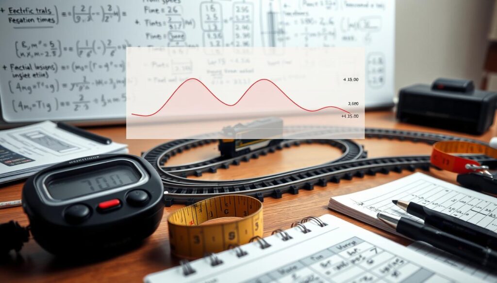
There are two main types of errors in our data. Systematic errors are the consistent troublemakers. If your track markers are 5 cm off, every distance measurement will be wrong by that same amount. It’s like a faulty unit conversion in your head—consistently translating meters to feet incorrectly.
Then there are random errors, the unpredictable guests. Your reaction time varies each trial. Maybe you blinked. Maybe the cat distracted you. These fluctuations create scatter in your data, like different musicians playing the same sheet music with slightly different tempos.
So how do we minimize this chaos? Through the scientific equivalent of practice makes perfect: repeated trials. One measurement is an anecdote. Ten measurements start telling a story. Thirty? Now you’re writing a novel with statistical significance.
Here’s your practical protocol:
- Run the same test at least 5 times under identical conditions
- Record every single time measurement, even the ones that look “wrong”
- Calculate the average (mean) of all your trials
- Note the range: fastest time to slowest time
The more trials you conduct, the more your random errors tend to cancel each other out. It’s the law of large numbers doing its magic trick. Your average becomes more reliable than any single measurement.
This brings us to reporting data properly. In real science, you never report just a number. You report the number plus its uncertainty. “The train’s speed was 0.85 ± 0.05 m/s” tells the whole truth. The ± 0.05 is your error bar—the confession of your measurement’s limitations.
Remember that pesky unit conversion practice from earlier? It matters here too. An error of 0.05 m/s becomes about 0.11 mph. Your uncertainty travels with your measurement through every calculation, like loyal but troublesome sidekicks.
Embrace the uncertainty. It’s not a failure; it’s honesty. The error bar isn’t a mark of shame—it’s a badge of scientific integrity. After all, perfect certainty is for mathematicians. The rest of us are just trying to get better thumb reflexes.
Challenge: Predict time for a 10-m run and test
Theoretical calculations are elegant, but reality can be humbling. This is where your spreadsheet meets the tracks. It’s a challenge that separates armchair theorists from hands-on scientists.
Your mission is to calculate how long your model train will take to travel 10 meters. You know its speed from previous experiments. Now, you’ll use the speed equation like a scientific crystal ball.
The math is simple: Time = Distance ÷ Speed. If your train averaged 0.45 m/s last time, it will take 10 ÷ 0.45 ≈ 22.2 seconds. Write this down. Circle it. This is your hypothesis, your mathematical bet against the universe.
Now, it’s time for the experimental verification. Set up a 10-meter track with clear markers. Place your train at the start, set the throttle, and grab your stopwatch. Take a deep breath. This is science in its purest form: make a prediction, then test it.
On your mark… get set… go! Start the stopwatch as the train passes the start and stop it at the finish. Record the actual time. Was it 22.8 seconds? 21.5? 23.1? The exact number doesn’t matter as much as what it tells you about your predictive power.
With your stopwatch data, compare prediction versus reality. Calculate the percentage error: [(Actual – Predicted) ÷ Predicted] × 100. A 0.6-second difference on a 22.2-second prediction is about 2.7% error. This is remarkably good for model railroading! This discrepancy isn’t failure; it’s data. It tells you about track conditions, motor consistency, and measurement limitations.
Why does this matter beyond toy trains? Every engineer, physicist, and project manager makes predictions based on known data. The Apollo missions, bridge constructions, and even your morning commute time estimate all use this same fundamental process: measure, calculate, predict, test. Your model train is teaching you the scientific method’s most valuable lesson.
The beauty of this challenge lies in its repeatability. Change the throttle setting and predict again. Try a different distance. Each experiment sharpens your predictive skills while revealing the subtle variables that affect real-world performance. This isn’t just math homework—it’s training for thinking precisely about an uncertain world.
Worksheet: Problems with step-by-step solutions
Ready for the fun part? Welcome to the worksheet section. Here, we dive into solving problems. We use the equation speed = distance/time to guide us.
Every problem is like a story. We show you how to solve them, step by step. It’s like having a math expert by your side.
Problem 1: The Commuter Express
A model train travels 8 meters in 4 seconds. What’s its speed in meters per second?
Step-by-Step Solution:
- Know the facts: distance = 8 m, time = 4 s.
- Remember the formula: speed = distance/time.
- Put in the numbers: speed = 8 m / 4 s.
- Do the math: 8 ÷ 4 = 2.
- State the answer: The train’s speed is 2 m/s.
See how easy it is? The equation does all the work. You just guide it.
Problem 2: The Scenic Route
Your train goes 3 feet per second. How long to cover 15 feet?
Step-by-Step Solution:
- Know the details: speed = 3 ft/s, distance = 15 ft.
- Need time. Change the formula: time = distance/speed.
- Plug in values: time = 15 ft / 3 ft/s.
- Do the math: 15 ÷ 3 = 5.
- Interpret: The units match (ft ÷ ft/s = s). Answer: 5 seconds.
Changing the equation is like solving a puzzle. Each piece fits perfectly.
Problem 3: The Cross-Country Challenge
A toy train does a 20-meter lap in 8 seconds. What’s its speed? Then, convert to miles per hour (1 m/s ≈ 2.237 mph).
Step-by-Step Solution:
- Find the average speed: speed = distance/time = 20 m / 8 s.
- Calculate: 20 ÷ 8 = 2.5 m/s.
- Convert: 2.5 m/s × 2.237 ≈ 5.59 mph.
- Context: That’s fast walking. Your train is almost jogging.
Converting units makes math real. Numbers become meaningful.
We start simple, add complexity, and add real-world examples. By solving these, you learn the basics of motion.
Try making your own problems. Change the numbers. The equation speed = distance/time always works. That’s the power of basic math.
Extension: Curves vs straights—does speed change?
We’ve mastered the straight and narrow. Now let’s bend the rules—literally. What happens when your Lionel or Bachmann locomotive meets a curve?
Real trains have a secret. Their wheels are coned, not cylindrical. This genius engineering lets them navigate bends without derailing. Märklin and Hornby models often replicate this design.
Set a curved section after your straight test track. Time a complete circuit. Compare this lap time to your straight-run data. Calculate the average speed for each segment.
The numbers might surprise you. The average speed frequently drops on the curve. Friction plays a bigger role. Forces push the train outward. It’s a hands-on lesson in circular motion.
This experiment pushes past simple calculations. It reveals the messy physics of real motion. Your model train becomes a tiny laboratory on rails.
That’s the final stop. Math projects with model trains show us the hidden language of motion. From measuring distance to graphing speed, we’ve decoded how things move. Now go test a curve.
