

What’s the point of running experiments if you can’t trust your results? I’ve seen students work hard, gather data for hours, and then doubt their findings. They ask, “How confident are you in that number?”
Here’s the truth. Without proper measurement error analysis, your project is just a show with fancy tools. Harvey Mudd’s physics department says it best: “No Information without Uncertainty Estimation!” Every measured value is surrounded by doubt.
Think about it. Mary has 3 brothers—that’s clear. Your circuit outputs 5.7 volts—that’s a measurement, full of experimental uncertainty.
The standard notation reveals the truth: measurement = (best estimate ± uncertainty) units. Saying “5.7 volts” is not enough. Saying “5.7 ± 0.2 volts” shows you get what you’re measuring.
Alan Greenspan once said, “It is better to be roughly right than precisely wrong.” Getting precision vs accuracy right isn’t just math. It’s about being honest. It’s the heart of the scientific method, where proving your work is more important than hoping for the best.
Tool choice resolution calibration routines
The meter stick on your lab bench has an opinion about reality, and it’s probably wrong. It’s not trying to be wrong, but it’s limited in a way most students don’t think about. Before you start measuring, you need to know that your tool doesn’t just affect your measurements. It defines the boundaries of what you can know.
Let’s talk about meter stick precision and what it really means. That ruler with millimeter markings looks precise, right? But the truth is, it can’t reliably measure anything smaller than about half a millimeter.
The lines themselves have thickness. Your eye has limits. The concept of instrument resolution describes this fundamental graininess—the smallest change your device can detect.
Electronic instruments make you think they’re more precise than they are. A digital balance accuracy reading of 17.43 grams looks more trustworthy than “about 17 grams,” doesn’t it? But those decimals might be lies dressed in precision’s clothing.
The device uncertainty matters more than the number of digits on the display. I’ve seen students trust a cheap scale’s third decimal place when the manufacturer’s own specifications admit uncertainty ten times larger. Reading the manual is unsexy, but it’s also not optional.
Consider the famous gold ring example that haunts physics labs everywhere. Weigh the same ring on two different balances: one reads 17.43 grams, the other reads 17.22 grams. Which one is telling the truth?
Plot twist: maybe neither. Without calibration standards, you’re just collecting expensive guesses. This is where systematic error sneaks into your experiment wearing a lab coat and pretending it belongs there.
| Instrument Type | Typical Resolution | Common Uncertainty Source | Calibration Frequency |
|---|---|---|---|
| Meter Stick | ±0.5 mm | Thermal expansion, wear | Annual verification |
| Digital Caliper | ±0.01 mm | Battery voltage, debris | Before each session |
| Electronic Balance | ±0.01 g | Vibration, air currents | Daily zero check |
| Digital Thermometer | ±0.1°C | Sensor drift, response time | Monthly against ice bath |
Calibration procedures aren’t just a formality. They’re your insurance policy against publishing garbage. The gold standard involves NIST-traceable references—objects or readings whose values are known with frightening precision because they’ve been compared against national standards.
For your purposes, this means using certified mass sets for balances or gauge blocks for calipers. Check the calibration before you collect data, not after you’ve already invested three hours in measurements. Trust me on this one.
Zero offset checking is the simplest calibration ritual, and students skip it with astonishing regularity. Place nothing on the balance. Does it read exactly zero?
If not, you’ve discovered a systematic error that would have contaminated every single measurement. Congratulations—you just saved yourself from retraction-level embarrassment. Temperature effects matter more than you think, and they can change your measurements.
Here’s where it gets clever: null methods are experimental judo moves that eliminate whole categories of measurement uncertainty. Instead of measuring an absolute value (which requires trusting your instrument completely), you measure a difference. Balance one unknown mass against another on a beam balance, and suddenly you don’t care about the balance’s absolute calibration—only its ability to detect inequality.
Instrument drift is the slow betrayal nobody warns you about. Electronic devices don’t stay calibrated forever. Sensors age, circuits warm up, and what read correctly this morning might be systematically off by this afternoon.
This is why professional labs obsess over calibration standards and re-check instruments throughout long experimental sessions. Your three-year-old multimeter might have opinions about voltage that differ significantly from reality’s consensus.
The practical implication? Your choice of measuring tool isn’t just about convenience or what’s available in the drawer. It’s a fundamental experimental decision that affects every calculation you’ll make.
Use a device with insufficient resolution, and you’re collecting noise. Use one without proper calibration, and you’re systematically wrong with great confidence. Neither option looks good on a lab report.
Repeat trials mean median stdev confidence
A single measurement is like judging a movie from one frame—technically data, practically useless. The universe doesn’t hand you perfect repeatability on a silver platter. Nature fidgets, instruments drift, and your hands shake just enough to make every trial slightly different.
This is where random variation enters the conversation. It’s not your fault, and it’s not a flaw in your technique. It’s the fundamental restlessness of reality itself, the cosmic truth that no two measurements are ever perfectly identical.
So you measure again. And again. And suddenly you’re not taking measurements—you’re characterizing a distribution.
The sample mean is your starting point. Add up all your measurements and divide by how many you took. The formula looks simple: x̄ = (x₁ + x₂ + … + xₙ)/N. It’s the center of your data’s story, the gravitational point around which everything else orbits.
But the mean alone is just coordinates without a map. You need to know how widely scattered your data points are. That’s where standard deviation comes in, quantifying exactly how much nature spreads your results around that central value.
Here’s the formula that matters: s = √[Σ(δxᵢ²)/(N-1)]. Each δxᵢ represents the difference between an individual measurement and the mean. Square those differences, add them up, divide by N-1, then take the square root. The result tells you the typical distance between any given measurement and the mean.
Why N-1 instead of N? Because we’re working with a sample of infinite possibility, not the entire population. That minus-one correction accounts for the fact that we’re estimating, not measuring the whole universe. It’s a subtle detail that makes your statistics honest.
Let’s work through real numbers. Say you measure a pendulum’s period five times: 0.46, 0.44, 0.45, 0.44, and 0.41 seconds. The sample mean comes out to 0.44 seconds. Calculate the deviations, square them, sum them up, and you’ll find a standard deviation of about 0.02 seconds.
That standard deviation describes individual measurements. But what about the mean itself? How confidently have you pinned down that 0.44-second average?
Enter the standard error of the mean. It’s always smaller than the standard deviation because averaging multiple measurements reduces uncertainty. The formula is simple: divide your standard deviation by the square root of N. More trials mean smaller error bars and tighter confidence.
| Measurement Number | Pendulum Period (seconds) | Deviation from Mean | Squared Deviation |
|---|---|---|---|
| 1 | 0.46 | +0.02 | 0.0004 |
| 2 | 0.44 | 0.00 | 0.0000 |
| 3 | 0.45 | +0.01 | 0.0001 |
| 4 | 0.44 | 0.00 | 0.0000 |
| 5 | 0.41 | -0.03 | 0.0009 |
Here’s where confidence intervals transform vague hunches into quantified certainty. One standard deviation captures about 68% of your measurements. If you report your pendulum period as 0.44 ± 0.02 seconds, you’re saying that roughly two-thirds of future measurements should fall between 0.42 and 0.46 seconds.
Double that error bar to two standard deviations, and you’ve bracketed 95% of expected results. This is the language of experimental confidence—numbers that let you say “I’m reasonably sure” with mathematical backing.
Consider measuring paper width across ten sheets. You get readings clustering around 31.19 cm with a standard deviation of 0.12 cm. That scatter isn’t sloppiness; it’s the reality of manufactured variation in paper cutting. Your data-driven training teaches you to expect this natural spread and quantify it properly.
Bean sprout heights offer another example. Measure twenty sprouts from identical seeds grown under identical conditions, and you’ll see variation. Some reach 8.2 cm, others barely hit 7.4 cm. The mean might sit at 7.8 cm, but the standard deviation tells the full story of biological variability.
The beautiful truth? If you could somehow measure infinitely many times, your sample mean would converge on the true mean. Each additional trial nudges you closer to reality. The standard error shrinks with √N, so quadrupling your trials cuts your uncertainty in half.
This statistical toolkit transforms you from someone who collects numbers into someone who makes defensible claims about nature. You’re not just reporting measurements anymore. You’re quantifying confidence, acknowledging uncertainty, and speaking the rigorous language of science.
Next time someone asks why you didn’t stop after one measurement, you’ll have an answer that goes beyond “because my teacher said so.” You’re characterizing distributions, not chasing single values. You’re mapping the landscape of possibility, one trial at a time.
Propagation of error rules for sums products ratios
When you mix several imperfect measurements to find a new quantity, things get interesting. You’ve measured mass with ±0.1 grams and volume with ±0.5 milliliters. Now, you want to find density.
Do the uncertainties just add up? Multiply? Or do they disappear into thin air?
Welcome to propagation of uncertainty, the math that follows error bars through calculations. This is where your high school algebra teacher’s warnings come in handy. Every calculation inherits uncertainty from its inputs, and ignoring this fact doesn’t make it disappear—it just makes your conclusions unreliable.
Two Approaches to Uncertainty Calculations
You have two main methods for tracking combined uncertainty through your calculations. Each has its place, and knowing when to use which separates careful experimenters from wishful thinkers.
The Upper-Lower Bound Method is straightforward but pessimistic. You calculate your result using the maximum possible values, then using the minimum possible values. The difference gives you the uncertainty range.
It assumes everything goes wrong simultaneously, which rarely happens in practice.
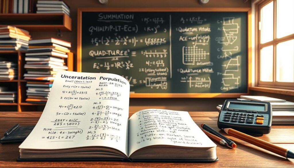
The Quadrature Method is more sophisticated and usually more realistic. It recognizes a key insight: independent random errors don’t add linearly. They combine in quadrature—you square each uncertainty, add those squares, then take the square root of the sum.
Why does this work? Because random errors tend to partially cancel out, not add up. It’s the statistical equivalent of acknowledging that Murphy’s Law has limits.
| Calculation Type | What Combines | Formula Pattern | When Dominant |
|---|---|---|---|
| Sums (A + B) | Absolute uncertainties | √(δA² + δB²) | Similar magnitude inputs |
| Differences (A − B) | Absolute uncertainties | √(δA² + δB²) | Small net result warning |
| Products (A × B) | Fractional uncertainties | √[(δA/A)² + (δB/B)²] × result | Poorest relative precision |
| Ratios (A ÷ B) | Fractional uncertainties | √[(δA/A)² + (δB/B)²] × result | Poorest relative precision |
The Critical Difference: Absolute vs Fractional Uncertainty
For addition and subtraction, you combine absolute uncertainties in quadrature. If you’re adding 10.0 ± 0.2 cm and 5.0 ± 0.1 cm, you combine the 0.2 and 0.1 directly: √(0.2² + 0.1²) = 0.22 cm.
Your result is 15.0 ± 0.22 cm.
For multiplication and division, you combine fractional uncertainties in quadrature. Fractional uncertainty equals uncertainty divided by the measured value. If you multiply 10.0 ± 0.2 cm by 5.0 ± 0.1 cm, you first calculate fractional uncertainties: 0.2/10.0 = 0.02 and 0.1/5.0 = 0.02.
Combine them: √(0.02² + 0.02²) = 0.028. Multiply by your result (50.0 cm²) to get 50.0 ± 1.4 cm².
Real Example: Density Calculation
You measure mass as 47.3 ± 0.1 grams and volume as 25.0 ± 0.5 milliliters. Density equals mass divided by volume. Which uncertainty matters more?
Calculate fractional uncertainties first:
- Mass: 0.1 / 47.3 = 0.0021 (0.21%)
- Volume: 0.5 / 25.0 = 0.020 (2.0%)
- Combined: √(0.0021² + 0.020²) = 0.020 (2.0%)
The volume uncertainty dominates completely. Your careful mass measurement barely affects the final uncertainty. This reveals where to focus your improvement efforts—get a better volume measurement tool, and your density uncertainty will drop significantly.
Ignore error propagation formulas, and you miss this insight entirely.
When Propagation Reveals Problems
Sometimes the quadrature method delivers bad news. If one input has terrible uncertainty, it will dominate your calculated result no matter how precisely you measured everything else. A single sloppy measurement can render five careful ones effectively worthless.
That’s not a failure of the math—it’s the math being honest with you.
Conversely, when you discover that two measurements contribute roughly equally to your combined uncertainty, you know you’ve balanced your experimental design well. Neither measurement is the obvious weak link. That’s the hallmark of thoughtful experimental work.
This is the calculus of experimental caution. The mathematics of intellectual honesty. You can’t fake precision through ignorance, and uncertainty calculations won’t let you pretend it’s true.
Graphs with uncertainty bars reading overlap correctly
Numbers in spreadsheet cells whisper their secrets, but graphs with uncertainty bars shout them across the room. I’ve seen students plot data without those critical little whiskers. This makes their measurements seem perfect, which is not science.
Let me show you how to make your graphs tell the truth.
Creating proper error bars visualization starts with knowing what uncertainty you’re representing. Are those bars showing standard deviation? Standard error? A 95% confidence interval?
Each choice changes how you interpret the graph. Most plotting software—Excel, Google Sheets, even Python libraries—lets you add error bars in a few clicks. But clicking buttons doesn’t guarantee understanding.
When you’re graphing experimental data, each point should sprout symmetrical whiskers. These extend above and below (for y-axis uncertainty) or left and right (for x-axis uncertainty). Sometimes both axes have uncertainty. In that case, your data points wear full crosses of doubt, which looks complicated but tells the complete story.
The Excel approach goes like this: plot your data normally, then select the data series, choose “Add Error Bars,” and input your uncertainty values. You can use fixed values, percentages, or reference specific cells containing your calculated uncertainties. Professional software like Origin or MATLAB offers more control, letting you customize bar cap sizes, colors, and whether they represent standard deviations or confidence intervals.
But here’s where students stumble: reading those bars correctly.
Two points with overlapping uncertainty bars don’t automatically agree. The degree of overlap matters enormously. If error bars barely kiss at their tips, those measurements probably differ significantly.
If they overlap by half their length or more? Now you’re talking about genuine agreement.
Non-overlapping bars send a clear message: these measurements represent different values, and you need to explain why. Did your experimental conditions change? Was there systematic error?
Is one measurement just wrong?
| Bar Relationship | Interpretation | Action Required |
|---|---|---|
| No overlap | Statistically different values; measurements disagree | Investigate experimental conditions, check for systematic errors |
| Slight overlap (tips touching) | Marginal agreement; borderline significance | Consider confidence level, possibly collect more data |
| Moderate overlap (50% or more) | Strong agreement; measurements consistent | Proceed with confidence in your results |
| Complete overlap (one bar inside another) | Excellent agreement; highly consistent measurements | Use combined data for analysis |
The confidence level behind your bars changes everything about overlap interpretation. Bars representing one standard deviation (68% confidence) require more overlap to indicate agreement than bars showing two standard deviations (95% confidence). This isn’t pedantic statistics—it’s the difference between claiming a discovery and admitting you found noise.
Now let’s talk about trendlines, because this gets delightfully counterintuitive.
A best-fit line might not pass through any of your error bars. That’s not failure—that’s chi-square minimization doing its job. The line represents the most likely relationship given all your data points and their uncertainties.
Individual points might scatter above and below, but if roughly two-thirds fall within one error bar of the line, you’ve got a good fit.
When you extract slope and y-intercept from your data plotting, those values carry their own uncertainties. Excel won’t tell you this automatically (because Excel wants you to feel confident, not informed). You need to calculate or estimate uncertainty in your fitted parameters.
Professional software often provides these values, showing results like slope = 2.34 ± 0.15. That uncertainty in the slope matters just as much as the slope itself when you’re testing hypotheses or comparing to theoretical predictions.
Here’s my practical workflow for creating honest graphs:
- Calculate uncertainties for each data point before opening plotting software
- Choose error bar type based on what you’re trying to communicate (usually standard deviation or standard error)
- Add error bars to your plot with clear legend indicating what they represent
- Fit trendlines only when appropriate, understanding that the line serves the data, not vice versa
- Extract fitted parameter uncertainties from software or calculate them manually
- Label axes with units and indicate confidence levels in captions
The visual impact of graphing experimental data with proper error bars visualization can’t be overstated. When your professor glances at your lab report, those whiskers communicate immediately whether your conclusion rests on solid ground or quicksand. A graph claiming a linear relationship with tiny error bars that barely touch the trendline? Convincing.
The same graph with honest error bars that dwarf your claimed trend? Time to collect more data or admit your hypothesis needs revision.
Chi-square fitting concepts provide mathematical rigor to what your eyes suspect. A reduced chi-square value near 1.0 suggests your error bars accurately represent your uncertainty and your model fits well. Values much larger indicate either underestimated uncertainties or a poor model.
Values much smaller? You’ve probably overestimated your uncertainties, which sounds safe but actually obscures real patterns in your data.
Making error bars communicate requires thinking about your audience. Will they understand that bars represent 95% confidence? Should you include a legend explaining your uncertainty calculation?
Is the visual difference between data sets obvious, or do overlapping bars create ambiguity that words must resolve?
Visual honesty in data plotting serves as epistemological discipline—a fancy way of saying it forces you to admit what you know and don’t know. When every measurement wears its uncertainty openly, overinterpreting noise becomes harder. Pattern recognition becomes fairer.
Your experimental story gains credibility precisely because you’re not hiding the messiness.
The goal isn’t creating pretty pictures for PowerPoint. It’s building trust through transparency. Those little whiskers transform scattered points into an honest representation of reality—uncertain, imperfect, but defensible.
When someone questions your conclusions, you can point to your overlap interpretation and say, “The data supports this within these bounds.” That’s not hedging. That’s science.
Case studies speed timing gate vs stopwatch sensor drift
One day, I found out a $500 photogate timer could be wrong in more ways than a $15 stopwatch. I was timing how fast a steel ball fell through a tube. The stopwatch said 0.5 seconds, but the photogate said 0.4573 seconds.
It turned out neither was right. But learning why each device failed taught me a lot about experimental design.
The stopwatch’s problem is obvious. Your reaction time is around 0.2 seconds on a good day. This delay is a common error in student experiments.
The photogate’s digital display makes it seem like it’s very accurate. But this accuracy is just an illusion.
| Measurement Method | Displayed Precision | Actual Accuracy | Primary Error Type |
|---|---|---|---|
| Human Stopwatch | ±0.01 seconds | ±0.15-0.25 seconds | Random (reaction time variability) |
| Photogate Timer | ±0.0001 seconds | ±0.01-0.05 seconds | Systematic (sensor lag, drift) |
| Video Analysis (60 fps) | ±0.017 seconds | ±0.02-0.03 seconds | Systematic (frame rate limitation) |
| Smartphone App Timer | ±0.001 seconds | ±0.10-0.20 seconds | Random (touchscreen lag varies) |
Precision shows how many decimal places a device can display. Accuracy shows how close it is to the truth. They’re like cousins who barely talk.
The photogate’s errors add up quickly. Electronics warm up in the first ten minutes, changing how the sensor works.
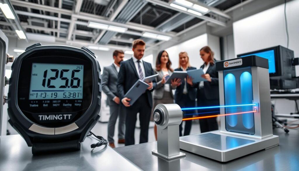
Temperature affects the photogate’s infrared beam. Air density changes with temperature, affecting light speed.
Microsecond-level changes are important. For most student experiments, they’re small. But they show a key principle: every measurement device responds to more variables than the one you’re trying to measure.
Environmental factors can ruin your experiment. A gentle breeze or footsteps can shake your setup.
I once spent three hours fixing a photogate problem. The issue was afternoon sunlight overwhelming the sensor. Moving the setup two feet fixed it.
Here’s a real-world error: sensor drift. Devices don’t stay the same over time. This affects their accuracy.
The photogate had a 2-millisecond delay. This is called hysteresis. For an object falling through the gate in 450 milliseconds, this error is 0.4%.
This delay wasn’t constant. It changed with temperature and how long the device was on. These errors aren’t in the manual.
To solve these problems, use different methods. I used three ways to measure the same drop:
- Photogate timing with infrared beam interruption
- High-speed video analysis at 240 frames per second
- Audio recording analyzing the impact sound timing
When different methods disagree, you see the errors each introduces.
The photogate was 8% faster than video analysis. This showed the beam placement or detection lag issues.
Audio analysis had the most variable results. Sound speed changes with temperature, and microphone placement caused geometric errors. But averaging different placements gave a better estimate than either method alone.
The truth about experimental design is that perfection is impossible. But knowing your errors is both possible and valuable. The goal is to characterize your error sources so thoroughly that someone else could replicate both your measurement and your uncertainty.
Different devices show different patterns. The stopwatch fails randomly. The photogate fails systematically. Random errors average out, but systematic errors do not.
Comparing methods is more important than trusting expensive equipment. A $500 timer with a 5% systematic error is less useful than a $15 stopwatch with random errors that cancel out over twenty trials.
The best design uses both types of measurement. Letting them disagree teaches you about what you’re not controlling. In real labs, what you’re not controlling is often more interesting than what you are.
How to write results with units and uncertainty a ± b
The way you report measurements shows if you know the difference between data and wishful thinking. After hours of careful work, your credibility depends on one simple format. If you get it wrong, you show you’re not competent before anyone reads your abstract.
The standard for measurement notation is simple: (measured value ± uncertainty) units. This is the promise you make to your reader about what you know.
But being simple doesn’t mean it’s easy. Precision has rules, and breaking them makes you look amateurish fast.
The Significant Figures Rule Book
Your uncertainty tells you how to write your measured value. The rule is: report uncertainty to one significant figure, maybe two if the leading digit is 1. Then, round your measured value to match that decimal place.
Writing 17.4327 ± 0.5 g is nonsense. Those extra digits pretend you know more than you do. The uncertainty of 0.5 g already shows you’re unsure at the tenths place, so why report to ten-thousandths?
The right way is 17.4 ± 0.5 g. It’s clean, honest, and defendable.
- Match your measurement’s decimal places to your uncertainty’s decimal places
- Round the measured value, don’t truncate it
- Never report more precision than your uncertainty justifies
- Use scientific notation for very large or very small values to maintain clarity
Consider 75.523 ± 0.5 g. Wrong. The uncertainty is in the tenths place, making everything else meaningless. A professional would write 75.5 ± 0.5 g, showing a fractional uncertainty of about 0.7%.
This principle applies to all measurements, from model trains measuring speed and distance to chemistry titrations. The format stays consistent because the logic does.
The Truth Table of Notation
Let’s see the difference between professional reporting standards and student mistakes. The table below shows correct notation versus common errors.
| Measured Value | Calculated Uncertainty | Incorrect Notation | Correct Notation |
|---|---|---|---|
| 17.4327 g | 0.5 g | 17.4327 ± 0.5 g | 17.4 ± 0.5 g |
| 0.003456 m | 0.0002 m | 0.003456 ± 0.0002 m | 3.5 ± 0.2 × 10⁻³ m |
| 125.789 s | 2.3 s | 125.789 ± 2.345 s | 126 ± 2 s |
| 9.876 N | 0.15 N | 9.876 ± 0.1532 N | 9.88 ± 0.15 N |
Notice how the correct column shows honesty? That’s not laziness. It’s intellectual honesty.
Percent Error: Your Reality Check
After writing your result right, you need to check how close you got to the expected value. That’s where percent error comes in, the standard for measuring how far off you were.
The formula is simple: (measured – expected)/expected × 100%. This calculation is used everywhere, from physics labs to engineering tests, and getting it right is key for credibility.
For example, if you measured a 50.0 g weight and got 49.3 ± 0.2 g, your percent error is: (49.3 – 50.0)/50.0 × 100% = -1.4%. The negative sign means you measured low, and the magnitude shows by how much.
Relative uncertainty works the same way but looks at your measurement’s internal precision. For that 49.3 ± 0.2 g measurement, the relative uncertainty is 0.2/49.3 × 100% = 0.4%. This shows your measurement’s uncertainty is less than half a percent of the value itself—very precise.
The Professional Standard
Your notation is more than just formatting. It shows your scientific maturity. When you write measurements with proper significant figures and precision, you show you understand the difference between measurement and certainty.
Sloppy presentation suggests sloppy thinking. In science, how you present your data is as important as the data itself. A measurement reported as 17.43 ± 0.01 g looks careful and controlled. The same measurement written as 17.4327 ± 0.5 g looks like you don’t understand your data.
Professional reporting standards aren’t just rules. They help us communicate uncertainty clearly, making promises about precision we can keep. Break these rules and you lose trust before anyone looks at your experimental design or statistical analysis.
The bottom line? Report uncertainty to one significant figure, round your measured value to match, and never pretend to know more than your measurements justify. That’s not modesty. That’s science.
Lab notebook habits timestamps diagrams data archiving
Think of your lab notebook as a time machine. It helps future you understand what you did today. It’s not for scrapbooking or journaling about physics. It’s a legal document, a scientific record, and your only defense against redoing experiments because you forgot details.
First rule of experimental records: write it down now, not later. Not when you get back to your dorm room.
Not after lunch when your memory has already started editing the data. The moment you observe something, that observation goes into your scientific notebooks. Why? Because 3.47 and 4.37 look awfully similar when you’re trying to reconstruct measurements from memory, and that decimal point makes all the difference.
Timestamps aren’t just for keeping track of time. They help spot systematic errors. Your sensor warms up.
The room temperature changes. Electronic equipment settles into different behavior patterns. When you notice unexpected variation in your data logging, timestamps let you correlate those changes with environmental factors or equipment behavior you might not have considered.
Steven Chu, who won a Nobel Prize for work that required exquisite experimental precision, once noted that mistakes are inevitable in research. The key is designing your research protocols to enable rapid correction. That means your notes need to contain enough detail that when something goes wrong—and it will—you can trace the problem back to its source without starting over.
Diagrams aren’t just for decoration. They’re maps showing how you connected components, oriented sensors, positioned shields, and controlled variables. Your written description might say “mounted the photogate on the vertical stand,” but your sketch shows exactly where on the stand, at what height, at what angle, and what else was nearby that might have interfered.
Archive your raw data before you touch it. Before you calculate anything, before you delete “outliers,” before you do anything that transforms the original measurements. Documentation practices demand this separation because you need to be able to go back and reanalyze with different assumptions if your initial approach reveals problems.
Record every calibration check and zero offset. Did you check the balance read zero before weighing samples? Write down what it actually read. Did you verify the timer against a known standard? Record both values.
These aren’t trivial details—they’re the foundation of your uncertainty analysis. If your zero reading drifts during the experiment, that drift becomes part of your systematic error budget.
Environmental conditions matter more than you think. Temperature, humidity, air pressure, nearby electrical equipment, foot traffic causing vibrations—all of these can affect measurements in ways that aren’t obvious until you’re trying to explain unexpected scatter in your results. Research protocols should include standard fields for recording these conditions, even when you think they don’t matter.
Good data logging supports what I call the circular process of experimental refinement. You design an experiment, execute it, analyze the results, and use what you learn to redesign intelligently. But that circle only works if your notes contain enough detail to identify what went wrong and what to change. When your uncertainty analysis reveals that timing precision is your limiting factor, you need to be able to look back and see exactly how you were timing events.
Keep track of uncertainties throughout the process, not just at the end. Note the resolution of each instrument as you use it. Record the spread in repeated measurements right there in your notebook, not just the average. When you estimate an uncertainty based on judgment—the width of a line, the precision of a manual alignment—write down your reasoning.
Your scientific notebooks are insurance against your own fallibility. We’re all fallible. Equipment fails, procedures change, collaborators remember things differently, and your own memory edits events in subtle ways. The only objective record is what you wrote down in real time, with sufficient detail that someone else could replicate your work.
Future you will judge present you by these records. So will your lab partners, your instructors, peer reviewers, and anyone who tries to build on your work. Make those records worthy of that judgment, because sloppy documentation doesn’t just make you look careless—it makes your results impossible to trust, no matter how good the underlying science might be.
Ethics report all trials prevent cherry picking
Let me tell you about a quiet fraud in student labs. You take ten measurements. Nine cluster nicely around a predictable value. One sits way out there, ruining your beautiful data set.
So you delete it. After all, something obviously went wrong, right?
Maybe. But unless you can document exactly what went wrong before you saw how that outlier affected your results, you’ve just committed a violation of scientific integrity. Welcome to the slippery slope of data manipulation.
Here’s the bright line you need to understand: mistakes are things you fix; errors are things you report. A mistake happens when you forget to zero your scale, drop a weight mid-measurement, or sneeze while timing. An error is the inherent uncertainty in your equipment and method that affects every measurement.
Cherry-picking data—excluding trials because they “don’t fit” your expectations—isn’t clever analysis. It’s fraud. Full stop. The distinction matters because one protects data ethics while the other destroys it.
When is outlier treatment legitimate? You need clear, documented reasons that exist independently of whether keeping or rejecting the point helps your hypothesis. Equipment malfunction you noticed during the trial? Document it immediately, then you can exclude that data point. Timer stopped mid-measurement? Write it down, exclude the trial.
But “it doesn’t match the others” isn’t a reason—it’s wishful thinking dressed up as quality control. Statistical tests exist for outlier treatment. Grubbs’ test, Dixon’s Q test, Chauvenet’s criterion—these provide objective criteria for exclusion.
Even then, you report that you excluded data and why. Transparency isn’t optional.
Let’s talk about “human error,” that meaningless cop-out students love to cite. Humans cause errors in specific, identifiable ways. Your reaction time adds 0.2 seconds to stopwatch measurements—that’s quantifiable uncertainty, not “human error.” You misread a graduated cylinder by estimating between tick marks—that’s reading error with a magnitude you can estimate.
Waving your hands and blaming “human error” tells me nothing about your experimental limitations. Name the specific source. Quantify its likely magnitude. That’s experimental honesty.
Here’s a table that should hang in every student lab. It distinguishes legitimate data exclusion from selective reporting:
| Legitimate Exclusion | Cherry-Picking (Fraud) | Documentation Required |
|---|---|---|
| Equipment malfunction observed during trial | Result “doesn’t look right” after collection | Timestamped note of malfunction before data analysis |
| Procedural error identified immediately | Outlier makes uncertainty bars inconveniently large | Description of error in lab notebook with witness |
| Measurement interrupted by external event | Data point contradicts your hypothesis | Record of interruption with specific details |
| Statistical test indicates outlier with objective criteria | Visual inspection suggests data “doesn’t fit” | Calculation showing test statistic and threshold |
Notice the pattern? Legitimate exclusions have three things: immediate identification, specific causes, and documentation that predates analysis. Everything else is just fraud with extra steps.
Calibration corrections are different from data manipulation. If you discover your thermometer reads 2°C high across all measurements, you should correct every reading by that systematic offset. That’s fixing a mistake. But you must document the calibration check and apply the correction uniformly—not selectively to readings that “need” it.
When your data contradicts your expectations, celebrate. You just learned something real about the world. Suppressing inconvenient results serves neither science nor your education. Your error bars should represent honest experimental assessment, not optimistic fantasizing about precision you didn’t achieve.
The principle underlying scientific integrity is simple: report all trials unless you can defend exclusion to a skeptical reviewer who assumes you’re trying to cheat. Because science is a trust-based system, and once you’ve been caught manipulating data, your career is effectively over.
I’m not exaggerating. Research integrity violations have ended careers of graduate students, postdocs, and tenured professors. The fabrication doesn’t need to be elaborate—selective reporting of trials is enough. Universities expel students for it. Journals retract papers. Professional societies revoke memberships.
Beyond career consequences, there’s intellectual integrity. You came to the lab to learn how the world actually works, not to confirm what you already believed. Every time you delete an inconvenient data point or fudge an uncertainty estimate, you’re lying to yourself about reality.
That’s not just unethical—it’s stupid. You’re paying tuition to be wrong in informative ways, to discover where your mental models break down. Experimental honesty is how you honor that purpose.
Here’s your action list for maintaining research integrity:
- Record all measurements immediately in permanent ink
- Note any procedural irregularities with timestamps as they occur
- Apply statistical tests for outliers with documented criteria
- Report excluded data with specific, defensible reasons
- Calculate error bars from all legitimate trials, not convenient subsets
Methodological transparency protects both your reputation and the scientific record. When you write up results, a skeptical reader should be able to reproduce your analysis and verify your conclusions. That means showing your work—all of it.
The uncomfortable truth? Most scientific fraud isn’t malicious. It’s students who don’t realize that “cleaning up” data crosses ethical lines. It’s researchers who convince themselves that one little exclusion doesn’t matter. It’s the slow accumulation of small compromises that erodes data ethics entirely.
You prevent it by drawing bright lines and refusing to cross them. Report all trials. Document exclusions before analysis. Let your error bars reflect reality, not wishful thinking. Treat every lab notebook like it might be read in court—because someday, it might be.
Science works because we trust each other to report what we actually observed, not what we wish we’d observed. Maintain that trust, and you’ll sleep better at night. Violate it, and you’ll spend your career looking over your shoulder.
Your choice. But choose wisely—because in science, your reputation is the only currency that matters.
Printable error analysis worksheet
Theory without practice is just philosophy. Practice without a plan is chaos. I’ve seen students rush through labs at 11 PM, searching online for “how to calculate standard deviation” while their data is scattered across many pages.
A good error analysis template can prevent this chaos. Your worksheet should lead you through the lab process before you get overwhelmed. Begin with the instrument’s specs and calibration checks. Record everything with timestamps and setup diagrams.
Make sure your data tables have uncertainty columns from the start, not as an afterthought. This way, you’ll avoid last-minute mistakes.
The best measurement protocol acts as your external brain. It reminds you to note environmental conditions and check for systematic errors. It also encourages you to run extra trials, which you’ll wish for later.
Your uncertainty checklist should cover instrument resolution, calibration drift, environmental factors, and human reaction time. This ensures you don’t miss any important details.
Have reference formulas on your worksheet, like standard deviation equations and confidence interval calculations. When you’re tired and just want to finish, these formulas help prevent big mistakes.
Print and use your worksheet often until it becomes second nature. It should eventually become unnecessary, showing you’ve mastered the process. This marks a big step from following rules to understanding their purpose.
