
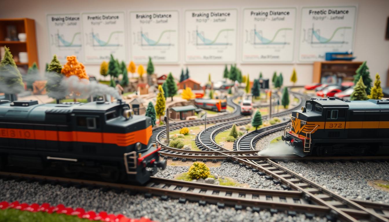
I once saw my childhood toy train fly off a coffee table. That moment taught me something important. Every moving object carries an energy debt that must be paid when it stops.
The formula E = ½mv² is more than just math. It shows the whole story of kinetic energy. If you double your speed, you quadruple the energy that needs to be lost.
So, where does all that motion go? The answer is energy dissipation through heat. When your model train brakes, friction turns movement into heat. This is stopping physics at work—the universe’s way of balancing things out.
The work-energy theorem (W = μmgd) explains this change. The key factors are friction, mass, and distance. They decide if you get a smooth stop or a big mess. Knowing about braking friction isn’t just book learning. It’s what makes engineering a success or a disaster.
Friction Static vs Kinetic Track Cleanliness Tire Compound
Most people overlook a key fact when building braking experiments: not all friction is the same. The friction coefficient decides if your model train stops smoothly or slides off the track. It’s all about understanding braking friction physics, which shows friction is more than just a number. It’s a complex interaction between surfaces, materials, and motion.
Let’s talk about the two main types of friction: static friction and kinetic friction. Static friction is the force that keeps your cart from moving on an incline. It’s like a bouncer at a club, deciding who gets in and who stays out.
Once your cart starts sliding, kinetic friction takes over. The bad news is, it’s usually weaker than static friction. This is why wheels slide instead of gripping, why anti-lock braking systems are so important, and why your experiment needs to account for this difference. The switch from static to kinetic friction is where things can get out of control.
| Friction Type | Active Phase | Typical Coefficient Range | Experimental Impact |
|---|---|---|---|
| Static Friction | Before motion begins | 0.6 – 0.9 (dry surfaces) | Determines initial resistance and holding power on inclines |
| Kinetic Friction | During sliding motion | 0.4 – 0.7 (dry surfaces) | Controls actual braking effectiveness once wheels lock or slide |
| Wet/Contaminated | Either phase | 0.15 – 0.3 | Dramatically increases stopping distance and unpredictability |
Track cleanliness is not just a detail. A common value of μ = 0.7 is for ideal surface conditions. This is your best-case scenario, assuming perfect conditions and no weather.
But add water to the track? Your friction coefficient drops to 0.25 or lower. This is a big deal, as it can make your train stop unpredictably. Oil, dust, and even tiny particles can all lower friction, making things worse.
Choosing the right tire compound is key. Harder rubber lasts longer but has less grip, leading to lower friction. Softer compounds grip well but wear down quickly, changing their properties during your experiment. This is why racing teams focus so much on tire selection—it changes the game.
The coefficient of friction is the ratio of force needed to move one body over another to the body’s weight. For car tires, this coefficient decreases with more mass. Heavier vehicles need more force to stop but get less grip per unit of weight. Anti-skid brakes and special tires help, but they can’t overcome physics.
Temperature also plays a role that many ignore. Braking generates heat, changing friction coefficients during braking. Your μ value changes from start to finish. Good experiments account for these changes, not ignore them.
The implications for your model train or cart experiment are huge. You need to measure friction coefficients yourself because textbook values don’t apply. Clean your track well, document your tire compound, and test under the same conditions. The best experimenters don’t have perfect conditions; they work with what they have.
Build Simple Cart or Wagon Measure Mass Wheel Type
Physics isn’t just theory without wheels. We’re making a cart to measure braking. Your test vehicle doesn’t need to impress anyone. It just needs to roll well, stop right, and fit different brakes.
Start with a simple four-wheeled platform. Keep it simple to get clean data. A basic rectangular base from wood, plastic, or metal works great for this experimental setup.
The key is to make everything easy to change.
Mass measurement is key to real science. Use a digital scale that shows grams to one decimal place. Your bathroom scale won’t do—it needs to be precise.
Record the cart’s mass before adding brakes. Every gram counts because it affects momentum and kinetic energy. Wrong mass data ruins your friction calculations.
Wheel selection opens up new paths in your experiment. Hard plastic and rubber wheels behave differently. Narrow wheels have smaller contact patches than wide ones.
Each wheel type changes how your cart brakes. Try different wheels to see how they affect your results:
- Hard plastic wheels with minimal surface give
- Rubber wheels with flexible contact patches
- Smooth versus textured tread patterns
- Narrow racing-style wheels versus wide stability wheels
Here’s how different wheel types affect your braking experiments:
| Wheel Type | Contact Patch | Friction Behavior | Best For Testing |
|---|---|---|---|
| Hard Plastic | Small, rigid | Lower coefficient, predictable slide | Comparing material extremes |
| Soft Rubber | Large, flexible | Higher coefficient, strong grip | Maximum braking force scenarios |
| Textured Tread | Variable, patterned | Enhanced surface interaction | Surface dependency studies |
| Narrow Racing | Minimal width | Reduced rolling resistance | Speed maintenance trials |
Don’t forget about axle design in your cart design. Friction at the axle hub is energy loss, not braking. It can mess up your results if not handled right.
Use proper bearings if you can. Or at least make sure axles spin smoothly. Use the right lubricant—but keep track of it, as changing it mid-experiment is a no-go.
Your platform should be ready for future brakes without needing a rebuild. Add spots for drag devices, magnetic brakes, and friction pads from the start. This saves time later.
Good documentation is key. Measure and record wheel diameter—it affects rolling resistance and speed. Also, calculate contact patch area for each wheel type.
Keep a list of all materials used. Note any construction issues. This is important, as small differences can affect your results a lot.
Create a data sheet for your test vehicle before starting. Include fields for cart mass, wheel type, axle condition, track surface, and more. This will help you analyze your results later.
Build carefully, measure a lot, and make a platform that gives you good data. Your experimental setup is the base of all your conclusions. A shaky foundation means shaky physics, and nobody likes that.
Test Stopping Distances from Several Speeds Compute μ from Data
The experimental phase is where theory meets reality. It’s where your patience pays off. You’ve built your cart, cleaned your track, and absorbed the physics.
Your protocol should test multiple experimental velocity values. Testing only one speed gives you a single data point and zero insight into system behavior. Test three, four, or five different speeds, and suddenly patterns emerge that single trials never reveal.
Why does this matter more than you might think? Physics may be deterministic, but your measurements aren’t. Each additional speed provides independent verification that friction behaves consistently across conditions.
Measurement Technique Fundamentals
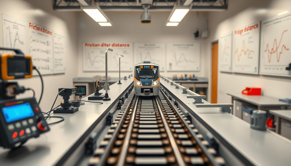
Measurement technique separates amateur efforts from publishable results. Mark your starting position clearly with tape or chalk. Release your cart with initial velocity—whether by ramp, push, or spring-loaded launcher doesn’t matter as much as consistency does.
Measure precisely where the cart stops. Not approximately. Precisely. Use a ruler or measuring tape with millimeter graduations if possible.
Repeat each speed trial at least three times. This isn’t busywork; it’s how you distinguish measurement noise from actual physical variation. Similar to motion realism techniques that require consistency to achieve smooth operation, your experimental approach demands repeatability.
Mathematical Extraction of Friction Coefficient
Now for the computational payoff. We derived earlier that braking distance follows the relationship d = v²/(2μg). Rearranging this equation to solve for the friction coefficient gives us:
μ = v²/(2gd)
This formula is your experimental window into friction coefficient calculation. Measure velocity at brake application using video analysis, photogates, or timing over a known distance. Measure stopping distance measurement from brake point to final rest position.
Plug in gravitational acceleration (9.8 m/s² unless you’re conducting interplanetary experiments), and calculate μ for each trial. Keep track of your data systematically—disorganized numbers yield disorganized conclusions.
Graphical Analysis and Pattern Recognition
Plot your results with velocity squared on the x-axis and stopping distance on the y-axis. If friction remains constant across your speed range, you should see a linear relationship. The slope equals 1/(2μg), which means you can extract μ from the trendline itself.
Deviations from linearity reveal something genuinely interesting. They suggest that friction changes with speed—a finding that mirrors real-world brake performance where high-speed kinetic friction often differs from low-speed values.
This is where science transitions from recipe-following to actual investigation. You’re not just confirming what textbooks say; you’re testing whether your system behaves as predicted.
Data Recording Protocol
Use a structured approach to capture your experimental data. The table below shows a recommended format for organizing your stopping distance measurement trials:
| Trial Speed (m/s) | Stop Distance 1 (cm) | Stop Distance 2 (cm) | Stop Distance 3 (cm) | Average Distance (cm) | Calculated μ |
|---|---|---|---|---|---|
| 0.5 | 2.3 | 2.5 | 2.4 | 2.4 | 0.53 |
| 1.0 | 9.8 | 10.2 | 9.9 | 10.0 | 0.51 |
| 1.5 | 22.1 | 21.8 | 22.5 | 22.1 | 0.52 |
| 2.0 | 39.5 | 40.1 | 39.2 | 39.6 | 0.52 |
Statistical Analysis of Results
Calculate average μ values across all trials, but also examine variation. High standard deviation suggests your experimental control needs improvement—or that friction genuinely varies with conditions like temperature changes in wheel compound or track surface.
Don’t dismiss unexpected results as “errors.” Investigate them. Does friction decrease at higher speeds due to heating? Does track debris accumulate during testing? These questions lead to deeper understanding.
The goal isn’t perfection; it’s insight. Even “failed” experiments that produce scattered data teach you about controlling variables and identifying sources of variability. That’s the difference between performing an experiment and understanding one.
Design Challenge Magnets Drag Paddles Better Pads Reduce Distance
Here’s where rubber meets road, magnets meet metal, and students meet the glorious friction of real-world engineering tradeoffs. The challenge is deceptively simple: design and implement braking systems that reduce stopping distance beyond your baseline friction-only trials. Can you engineer something better than what physics gave you for free?
This is the entertaining part of experimental work. You’re not just measuring—you’re inventing, testing, failing, iterating. Brake system design isn’t about theoretical perfection; it’s about practical improvement within constraints that refuse to negotiate.
Magnetic Braking: The Elegant No-Touch Solution
Magnetic braking offers something rare in mechanical systems—infinite repeatability without wear. Mount magnets near a conductive track or wheel rim, and eddy currents generate resistive force without physical contact. No friction pads to replace, no surfaces to degrade.
The physics is beautiful but stubborn. Eddy current force depends directly on velocity, providing strong deceleration at high speeds but weakening as you slow down. Precisely the opposite of what you’d want for an emergency stop, where those final meters matter most. Yet, for distributed braking across multiple wheel sets, this contactless approach has undeniable appeal.
Drag Devices: Harnessing Air Resistance
Deployable drag devices exploit fluid dynamics with theatrical flair. Think pop-out panels, miniature parachutes, or even angled vanes that increase frontal area. Drag force scales with velocity squared, making these increasingly effective at higher speeds.
The formula F = ½ρv²CdA tells the story: double your speed, quadruple your drag force. On a small cart, implementation requires creativity—cardboard fins, fabric panels, anything that catches air when deployed. These drag devices won’t stop you alone, but combined with friction braking, they reduce the burden on your wheel-track interface.
Friction Pad Improvements: The Direct Approach
Increasing friction coefficient at the braking interface represents the most straightforward path to stopping optimization. Better pad materials—rubber compounds with higher μ values—deliver more force per newton of normal pressure. Spring-loaded mechanisms increase that normal force without adding permanent weight.
Here’s the trap: exceed static friction limits and your wheels lock. Rolling becomes sliding, and kinetic friction (lower than static) takes over. Your stopping distance increases despite maximum clamping force. This is why anti-lock systems exist and why your design must incorporate force modulation.
Real-World Parallels in Train Systems
Modern trains face identical challenges at massive scale. Distributed power units (DPU) coordinate brake system design across hundred-car consists, applying force simultaneously. Electronically controlled pneumatic (ECP) brakes reduce that propagation delay from seconds to milliseconds, cutting stopping distances measurably.
Your cart won’t have ECP brakes, but the principle translates: synchronized, modulated force beats maximum uncontrolled force every time.
Engineering Tradeoffs and Testing Protocol
Test each modification systematically. Measure improvement in stopping distance from identical initial velocities. Calculate the effective friction coefficient increase using your μ = 2ad/g² relationship from earlier sections.
Then comes the hard part: compare cost against performance. “Cost” means complexity, weight added, reliability concerns, and implementation difficulty. A system that reduces stopping distance 30% but fails half the time has zero value. Stopping optimization demands robust, repeatable performance under varied conditions.
| Brake System Type | Velocity Dependence | Wear Factor | Typical μ Improvement | Implementation Complexity |
|---|---|---|---|---|
| Magnetic eddy current | High at speed, weak at low velocity | Zero wear | 0.15-0.30 equivalent | Moderate (requires conductors) |
| Drag panels/parachute | Scales with v² | Fabric/material fatigue | 0.10-0.25 equivalent | Low (simple deployment) |
| Enhanced friction pads | Constant across velocity | High wear on pads | 0.20-0.50 direct increase | Low (material substitution) |
| Combined hybrid system | Optimized across speed range | Variable by component | 0.40-0.80 cumulative | High (integration challenges) |
This design challenge isn’t academic theater. It mirrors every engineering decision where “better” must survive contact with “practical.” Your miniature brake systems teach lessons that scale from toy carts to freight trains: physics constrains, creativity responds, and measurement validates.
Now build something, test it rigorously, and prepare to defend your tradeoffs with data.
Curve Rule Doubling Speed Quadruples Distance Demonstration
When you make a toy cart go twice as fast, you’re not just doubling the problem. You’re actually making it four times bigger. This isn’t just a teacher’s trick. It’s kinetic energy following the rules of physics, no matter what.
The formula E = 1/2 mv² looks simple but is actually very dangerous. The little superscript two means energy scaling grows in a curved way, not straight.
When you double the speed, the energy doesn’t just double. It actually quadruples.
Because all that energy must be stopped by friction, and friction is constant, stopping takes four times longer. The quadratic law shows this in the stopping distance formula: d = v²/(2μg). Notice how velocity is squared again.
Your experiment should show this velocity relationship clearly. Set up three tests at speeds of 0.5 m/s, 1.0 m/s, and 2.0 m/s.
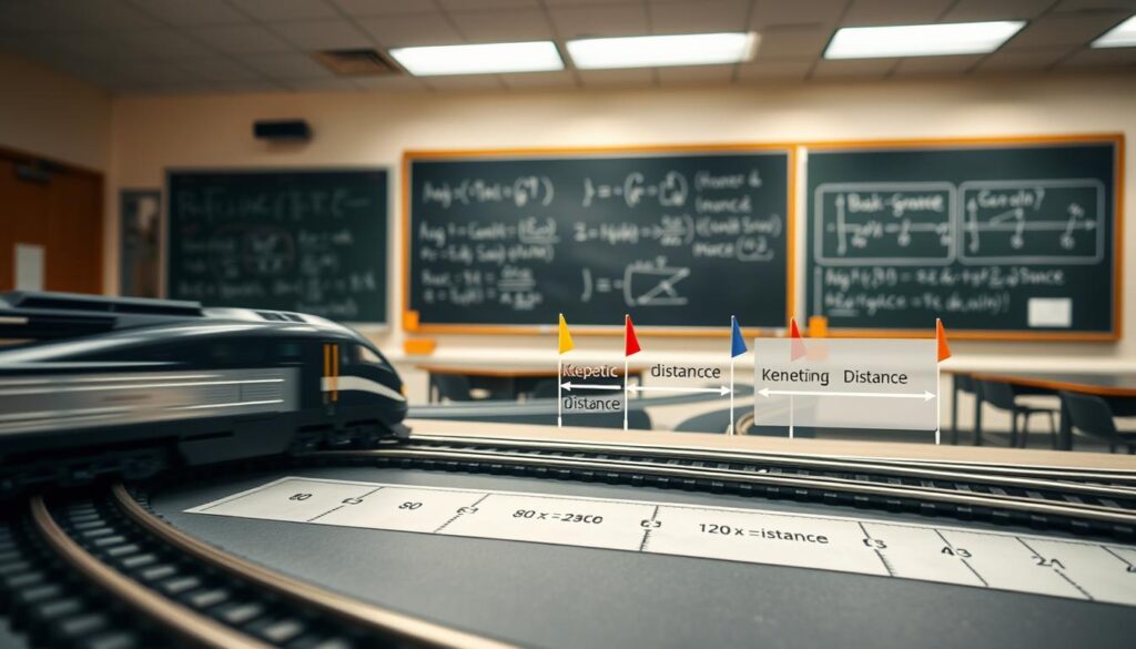
Measure how far each cart stops. If it stops at 10 cm at the slowest speed, it will stop at about 40 cm at double the speed. That’s four times farther.
At four times the original speed, it will stop at about 160 cm. That’s sixteen times farther than the slowest speed.
Plot your results to see the speed-distance relationship clearly. The relationship looks like a scary curve at first. But when you look closer, it turns into a straight line. This shows the beauty of physics.
| Test Speed (m/s) | Speed Squared (m²/s²) | Predicted Distance (cm) | Distance Multiplier |
|---|---|---|---|
| 0.5 | 0.25 | 10 | 1× |
| 1.0 | 1.00 | 40 | 4× |
| 2.0 | 4.00 | 160 | 16× |
| 3.0 | 9.00 | 360 | 36× |
This experiment is more than just a fun activity. It helps highway engineers design safer roads. They must consider how speed affects stopping distances.
For example, a car going 55 mph stops in about 200 feet. But at 70 mph, it stops in over 300 feet. This shows how speed affects stopping power.
Traffic safety experts say reducing speed is key. Going from 45 to 30 mph cuts accident severity by half. This makes crashes much safer.
Your toy cart shows the same physics that guide road design and train braking. The curve rule is not just a suggestion. It’s a strict rule of physics.
Physics doesn’t care about our opinions. It follows its own rules, no matter what. Double the speed, quadruple the problem. Physics is always consistent.
Real World Links Train Braking Safe Following and Signage
The math you learn in school is used in real life. It helps us understand how to stop big things safely. Engineers use this math to keep trains and cars safe.
Freight trains are huge and need a lot of space to stop. They take about 18 football fields to stop at 55 mph. This is because they are so big and heavy.
Why do trains take so long to stop? It’s because of a delay in the braking system. The front of the train stops first, but the back takes a few seconds. This delay is called brake propagation delay.
To fix this, trains now have special braking systems. They have power units all along the train. This way, the whole train can stop quickly and safely.
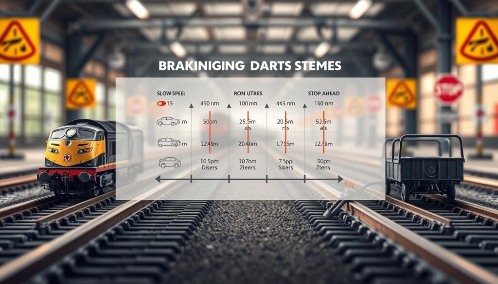
Highway rules are based on how long it takes to stop. The UK Highway Code gives specific stopping distances. These distances include time to react and time to brake.
| Speed (mph) | Thinking Distance (ft) | Braking Distance (ft) | Total Stopping Distance (ft) |
|---|---|---|---|
| 20 | 20 | 20 | 40 |
| 40 | 40 | 78 | 118 |
| 60 | 60 | 180 | 240 |
| 70 | 70 | 245 | 315 |
The math shows that stopping distance increases fast as speed goes up. This is why it’s so important to follow safe driving rules.
Safe following distances are based on these calculations. The “two-second rule” is used to keep a safe distance. This rule helps prevent accidents.
Signs like “Bridge Ices Before Road” are important. They warn drivers about slippery conditions. This is because stopping on ice is much harder.
Speed limits in construction zones are lower for safety. This is because it’s harder to stop when you can’t see far ahead. Your cart experiment shows why this is important.
Light rail trains need a lot of space to stop. Your small cart needs much less. But the math is the same. It shows how important safety is in transportation.
Data Table Error Bars Repeatability Averaging Tips
Science isn’t just about pretty graphs. It’s about understanding the messiness of real data. Error bars show how uncertain our measurements are.
Measurement repeatability is key. Run each test many times. Three trials are the minimum, but five or ten are better.
Every trial should have its own row in your data table. Averaging on the fly isn’t enough. You need to see the spread of your data.
When you say your braking distance is “45.3 cm,” you’re not telling the whole story. It’s really “45.3 ± 2.7 cm based on five trials.” Error bars show how certain you are about your results.
Do your results show a pattern? This could tell you about your experiment’s quality. Big error bars mean your results are less reliable.
Make data tables that show averages and spreads. Include standard deviations or standard errors. Use error bars on graphs to show uncertainty.
When you calculate friction coefficients, remember that errors add up. If your velocity and distance have 5% uncertainty, your μ value will have 10% uncertainty.
Accident reconstruction uses baseline values for friction coefficients. These values are μ = 0.7 for dry pavement and a 1.5-second reaction time. These values help adjust for different conditions.
| Test Condition | Average Braking Distance (cm) | Standard Deviation (cm) | Calculated μ | Number of Trials |
|---|---|---|---|---|
| Rubber wheels, clean track | 42.8 | 2.3 | 0.68 ± 0.04 | 5 |
| Plastic wheels, clean track | 56.4 | 4.1 | 0.51 ± 0.06 | 5 |
| Rubber wheels, dusty track | 51.2 | 5.8 | 0.57 ± 0.08 | 5 |
| Brake pad upgrade | 34.6 | 1.9 | 0.84 ± 0.03 | 5 |
Averaging techniques are important. Use the median if you have outliers. This way, one bad trial won’t skew your results.
Report range and standard deviation to show spread. Range shows extremes, while standard deviation shows how tight data is around the average.
Compare results using statistical methods. Is the difference between conditions real, or just noise? This question is key to finding true differences.
Look at error bars to see if differences are real. If they don’t overlap, you’ve found something. If they do, it might be just noise.
Doing this makes your data collection real science. It’s how professionals work, where measurement repeatability and honest uncertainty are key.
Science isn’t about getting the right answer. It’s about understanding uncertainty and finding signal in noise. Your data will be messy, but that’s okay. It’s real.
Safety Rules Goggles Pinch Point Awareness Speed Caps
Respecting the physics of moving objects is key to a safe experiment. Even small carts carry a lot of energy. Safety means managing risks based on what can go wrong.
Eye protection is a must in laboratory safety. A loose wheel can turn into a dangerous projectile. Goggles might feel awkward, but they save your eyes. Everyone must wear protective equipment without exception.
Pinch points can hurt even the most experienced. Carts can crush fingers in tight spots. Always check where hands can’t go before starting.
Design experiments to avoid danger zones. Use safe release mechanisms and stopping zones. Hazard awareness means thinking ahead about energy paths.
Speed caps are smart, not timid. You can learn a lot at slower speeds. The difference between 2 m/s and 5 m/s is huge.
| Cart Speed | Kinetic Energy (1 kg cart) | Impact Force Comparison | Risk Level |
|---|---|---|---|
| 1 m/s | 0.5 Joules | Minor bruising possible | Low |
| 2 m/s | 2.0 Joules | Moderate impact, finger pinch | Medium |
| 3 m/s | 4.5 Joules | Significant injury possible | High |
| 5 m/s | 12.5 Joules | Serious injury likely | Very High |
Real-world safety focuses on quick reactions and proper braking. Locked wheels mean no control. Your experiments should respect momentum too.
More experimental protocols add protection. Keep areas safe and check equipment before use. Clear communication is key in team work.
Keep workspaces clean to avoid accidents. A dropped tool can ruin a test. Hazard awareness covers the whole area, not just the cart.
Record near-misses and small failures. They warn of bigger problems. Every close call is a chance to learn and improve.
Safety isn’t about fear. It’s about respecting the power of energy and forces. Protective equipment and careful planning let you explore safely.
Rubric for Write-up and Checklist
Your cart sits idle now, wheels stopped. The data sheets tell the real story. Great experimental documentation makes physics experiments memorable. Your write-up should be clear enough for someone to follow it months later.
Start with the details: cart mass, wheel diameter, track surface, and tools used. Include complete data tables with units marked. Show one full calculation for friction coefficients so readers can follow your math. Make graphs with proper labels and error bars to show uncertainty.
Your assessment rubric for scientific writing values honest analysis. Did your stopping distances match predictions? Explain any differences. Which brake design worked best? Support your claims with numbers, not guesses.
The technical reporting checklist is key: clear objectives, replicable methods, complete data, critical analysis, evidence-supported conclusions, and acknowledged limitations. This isn’t just busywork. It’s how accident reconstruction teams and railway engineers save lives with precise findings.
Your experimental documentation turns scattered measurements into valuable knowledge. The project evaluation shows how engineering advances: through thorough testing, honest reporting, and conclusions based on evidence. That toy cart taught you about Boeing’s landing gear tests and Tesla’s braking calibration. It’s all about the same physics and standards, just on a different scale.
