
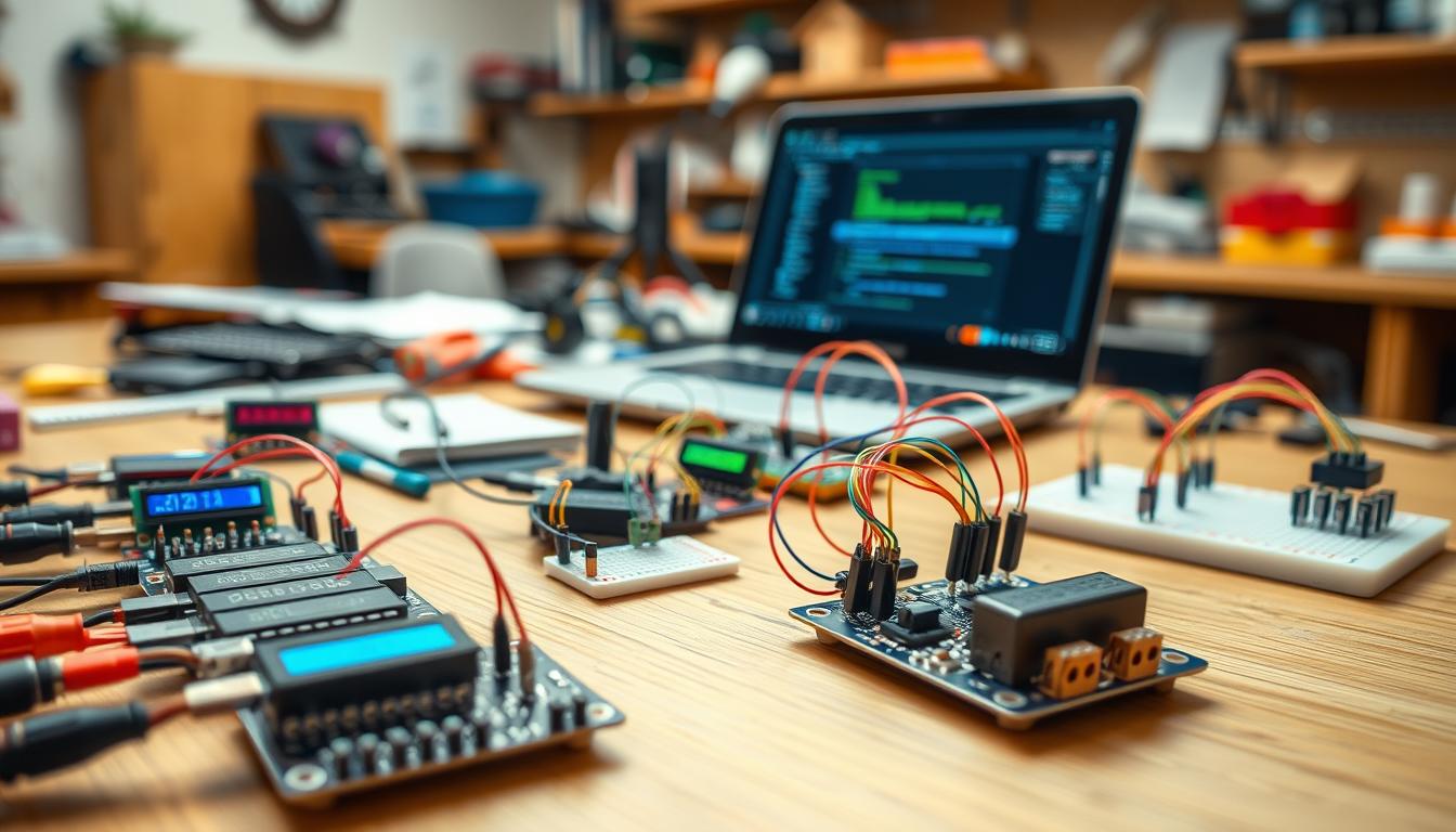
So you want to let students play with measurement tools? Brave soul. We’re not talking about old oscilloscopes anymore. We’re empowering the next generation to measure the world, not just read about it.
Modern sensors data logging is easy for everyone to use. You can start with a $10 setup or go for a more expensive one. The basics are the same.
Students can connect their own Arduino sensors to measure temperature, pressure, and speed. Seeing numbers on a screen shows them the universe is real and measurable.
This guide shows how to build DIY data acquisition systems in schools. It’s about combining maker culture with science. Even when things go wrong, it’s a chance to learn.
We’ll look at educational sensor platforms and how to measure right. Teaching students to measure is important. But it’s even more important to teach them why.
Wiring diagrams thermocouple amp pressure sensor Hall pickup
Connecting wires can be tricky. It’s easy to make mistakes that can damage your project. A small error can turn your device into a faulty one.
Thermocouples need careful handling. They produce very small voltages that need amplification. Without it, your device won’t work right.
Your thermocouple amplifier boosts the voltage so your device can read it. Make sure to connect the wires correctly. Use 3.3V or 5V power as needed.
Pressure sensors also need careful wiring. They output voltages that change with pressure. Some even use I2C for easier connection.
Check your pressure sensor’s wiring carefully. Most need three connections: power, ground, and signal. I2C sensors need four and follow specific rules.
Hall sensors detect rotation. They work well with things that spin. Place a magnet on the spinning part and connect the Hall sensor nearby.
Wiring a Hall sensor is simple. You need three connections:
- VCC: Power supply (usually 3.3V or 5V, verify your specific model)
- GND: Ground connection to microcontroller ground rail
- OUT: Digital signal output to interrupt-capable pin (D2, D3 on Arduino Uno)
I2C connections can be tricky. They need four wires. Don’t forget to cross the data lines.
Standard I2C connections are:
- SDA (data line) connects to A4 on Arduino Uno, but verify your board’s pinout
- SCL (clock line) connects to A5 on Arduino Uno
- VCC provides power at the correct voltage level
- GND establishes common ground between all devices
Make sure to cross the I2C wires correctly. This is important for modules with reversed pinouts.
UART connections also need precision. When using a CP2102 USB-to-serial adapter, follow these steps:
| CP2102 Pin | Logger Pin | Function |
|---|---|---|
| DTR | DTR | Data Terminal Ready (auto-reset) |
| RXD | TXO | Receive crosses to Transmit Out |
| TXD | RXI | Transmit crosses to Receive In |
| GND | GND | Common ground reference |
| 3.3V | VCC | Power supply (match voltage!) |
Matching voltage levels is critical. Using the wrong voltage can damage your sensor. Always check the voltage before connecting.
Real-time clock modules have alarm outputs. The SQW pin can wake your microcontroller. Connect it to D2 and set up your interrupt service routine.
Dewesoft systems handle signal conditioning for you. But if you’re building from scratch, you’re the signal conditioning engineer.
Common ground is key for all your components. It keeps everything working together. Without it, you’ll face noise and errors.
Students often make mistakes. They might reverse polarity or use the wrong voltage. Be prepared to replace sensors. It’s a valuable lesson.
Sampling rate Nyquist how fast is enough for piston cycle
Before you start, you must decide how fast to sample. This choice can make or break your data plot. It’s not just about speed; it’s about getting real insights.
Sampling theory, based on Harry Nyquist’s theorem, is key. It says you need to sample at least twice the highest frequency you’re measuring. If you don’t, you’ll get fake data through aliasing.
Let’s look at an engine example. A four-stroke piston at 3,000 RPM has a frequency of 50 Hz.
To capture this, you need at least 100 samples per second. But, if you sample at exactly 100 Hz, your data will look simple.
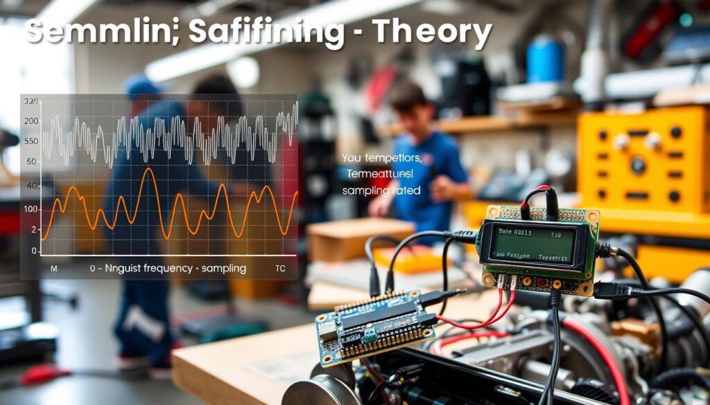
Professional engineers usually sample five to ten times faster than needed. This isn’t just being careful; it’s necessary.
Oversampling helps see details and apply filters well. For serious work, like studying pistons or vibrations, you need kilohertz rates.
But, for simple experiments, like measuring temperature or pressure, slower sampling works. This is because these changes happen slowly.
The e360 logger’s one-second alarm is useful for these slow changes. It helps students focus on important signals. Sampling too fast can lead to big data problems.
Different projects need different sampling rates. Some systems are made for low, medium, and high-speed recording. But, remember, faster sampling means more data and memory issues.
So, how do you choose? Start with the physics of your project, not just your equipment.
| Measurement Type | Typical Frequency Range | Minimum Sampling Rate | Recommended Rate |
|---|---|---|---|
| Temperature change (classroom) | 0.001 – 0.1 Hz | 0.2 Hz (5 seconds) | 1 Hz (1 second) |
| Pressure fluctuation (slow) | 0.01 – 1 Hz | 2 Hz | 10 Hz |
| Piston cycle at 3,000 RPM | 50 – 500 Hz | 1,000 Hz | 5,000 Hz |
| Vibration analysis | 10 – 10,000 Hz | 20,000 Hz | 50,000 Hz |
This table is a guide, not a rule. Your project might need more or less sampling. The key question is: what’s the fastest thing happening in your system?
For beginners, one-second sampling is often enough. It’s great for learning the basics of measurement. You’ll learn to measure before you try to measure faster.
But, for detailed work on pistons or sounds, you need special tools. Each tool is best for its specific task. A hammer isn’t wrong for not cutting; it’s just not a saw.
Choosing the right sampling rate is critical. Too slow and you miss important details. Too fast and you get overwhelmed by data. The goal is to find a balance that works for your project.
For most educational projects, sampling rates between one and hundred samples per second are good. Faster rates require special hardware and a clear reason for it.
Remember, the right sampling rate helps you focus on what’s important. It’s not about being fast; it’s about being accurate.
Calibrate with boiling ice and hand pump compare to analog
Before you trust a single temperature measurement, let’s talk about ice water and the democratic beauty of reference points. Your sensor might arrive with impressive specifications and a glossy datasheet. But shipping, handling, and that inevitable moment when someone tests if the soldering iron is hot enough all conspire against factory promises.
Ice water and boiling water represent the most accessible temperature standards known to science. At sea level, crushed ice in distilled water stabilizes at precisely 0°C. Vigorously boiling water hits 100°C, assuming you’re not conducting experiments on a mountaintop where atmospheric pressure becomes an inconvenient variable.
Here’s the reality check your thermocouple desperately needs. After manufacturing, shipping across continents, and casual mistreatment in a student workspace, that factory calibration certificate means approximately nothing. Verification becomes not just prudent but essential for any measurement you plan to defend in a lab report.
The classroom methodology is beautifully simple. Prepare crushed ice in distilled water and stir thoroughly until thermal equilibrium arrives. Your sensor should read 0°C, give or take atmospheric pressure and altitude corrections. Compare the reading, note the offset, and either correct in software or acknowledge the systematic error in your uncertainty analysis.
For pressure sensors, a hand pump with an analog dial gauge provides similar ground truth as effective calibration methods. The term “analog” here refers to mechanical dial gauges with springs and gears, not your uncle’s vinyl record collection. These mechanical references carry institutional trust built over decades of industrial use.
The beautiful irony? Modern digital sensors often demonstrate superior precision compared to their analog predecessors. Yet we rely on analog reference points for calibration because mechanical pressure gauges and mercury thermometers have earned credibility through centuries of consistent performance.
Consider the data from real implementations. The Cave Pearl Project documented NTC thermistor calibration achieving noise variation of just ±0.015°C in classroom conditions. That produces graph lines approximately 0.03°C thick, which represents exceptional sensor accuracy for educational settings. Measurements from Vaisala data loggers trace back to SI units through national metrology institutes or ISO/IEC 17025 accredited laboratories.
Understanding the boiling water method for thermometer calibration helps students grasp why these simple techniques remain relevant even in the digital age. The method’s accessibility makes calibration a routine practice, not an intimidating laboratory ritual requiring expensive equipment.
But here’s the practical consideration most datasheets ignore. Altitude matters more than manufacturers admit. Subtract approximately 1°C from your boiling point for every 300 meters above sea level. Physics doesn’t respect your convenience, and water’s boiling point follows thermodynamic laws, not your project deadline.
Students need to internalize one critical concept: measurement without calibration is just expensive guessing. That ±0.03°C uncertainty in a classroom project is absolutely acceptable when NIST-traceable temperature standards cost more than your entire course budget. Professional calibration services exist for critical applications, but student builders work within different constraints.
| Calibration Method | Equipment Cost | Achievable Accuracy | Suitable For |
|---|---|---|---|
| Ice Bath (0°C) | $5-10 | ±0.5°C | Thermocouples, thermistors |
| Boiling Water (100°C) | $5-10 | ±1.0°C (altitude dependent) | Temperature sensors |
| Hand Pump with Gauge | $50-150 | ±2% full scale | Pressure transducers |
| NIST-Traceable Lab | $200-500 per sensor | ±0.01°C | Critical medical/aerospace |
The e360 project using 10k 3950 NTC thermistors with 16-bit integer variables demonstrates practical limitations. These thermistors exceed the 65,535 ohm limit at approximately -12°C, which means your measurement range has physical boundaries regardless of your Arduino’s computational enthusiasm.
Documentation separates legitimate science from educated guessing. Record your calibration methods with embarrassing detail. Write down the date, temperature, humidity, atmospheric pressure, and which analog gauge you trusted. Future you, writing the final report at 2 AM, will appreciate past you’s obsessive note-taking.
Accept your limitations with grace. A thermocouple calibrated in a classroom with ice water and a hand pump will never match laboratory-grade instruments. That’s fine. Your goal is understanding measurement principles and quantifying uncertainty, not competing with national standards laboratories.
Compare your digital readings against analog references and embrace the philosophical question: which one is actually “right”? The analog gauge might have a lineage dating to 1950s German manufacturing. Your digital sensor boasts 16-bit resolution but could have drifted.
The answer lies not in trusting one over the other but in understanding both. Cross-reference multiple measurements, document systematic offsets, and report your sensor accuracy with honest uncertainty bounds. That’s the difference between data and mythology, between engineering and wishful thinking.
Know your tolerances. Document your methods. Accept your limitations. Then build something.
Log to SD card or Bluetooth graph in Sheets or Python
You’ve captured a mountain of sensor readings—now what? The world of student builders splits into two groups. There are those who prefer SD card logging for its tangible storage. Others want real-time streaming like their favorite shows.
SD cards are simple and hold a lot of data. Even old 2GB cards can store hundreds of thousands of readings. But, they make waterproofing harder and use a lot of power.
The e360 logger takes a different approach. It stores data in onboard memory, not on removable cards. This limits memory, but you can expand it if you plan ahead. Download data via USB when you get home.
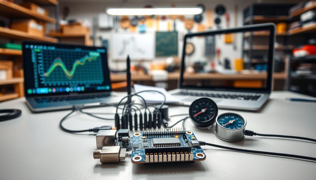
Modern Bluetooth modules change the game. They stream data to your phone, laptop, or cloud in real-time through wireless data transfer. This is great for getting feedback fast or when you can’t get the logger often.
The Cave Pearl code base has some limits. Sensor outputs are 16-bit integers, and each record can be 1, 2, 4, 8, or 16 bytes. These rules help you design data structures efficiently from the start.
| Storage Method | Capacity | Power Consumption | Real-Time Access |
|---|---|---|---|
| SD Card | Hundreds of thousands of readings | Moderate during writes | No |
| Onboard Memory | Limited but expandable | Minimal | No |
| Bluetooth Streaming | Cloud-limited | Higher continuous draw | Yes |
Once data is out of the logger, how you show it matters. Google Sheets makes plotting easy for spreadsheet experts. Just import CSV, pick columns, and insert a chart.
Python graphing with matplotlib or plotly offers endless customization for those who code. Turn raw data plot sequences into professional-looking figures. The learning curve is steep, but the results are worth it.
Systems like Dewesoft work with many formats and platforms. Vaisala’s viewLinc software uses OPC UA Server for integration, with API for database access. These solutions are powerful but complex, often too much for student projects.
The best choice depends on your needs. Consider these factors:
- Project duration and total expected readings
- Available power budget for your sensor package
- Need for real-time monitoring versus batch analysis
- Team comfort level with coding versus spreadsheet tools
- Physical access constraints to retrieve logged data
Start simple and add complexity as needed. A student can begin with Google Sheets data visualization and move to Python later. The most advanced system is useless if no one sees the data.
Remember, your storage strategy can change. Many projects start with SD cards and add Bluetooth later. It’s better to start small and grow than to do nothing.
Derive rpm average pressure simple work estimates
Students often find a gap between voltage readings and understanding mechanical work. Your Arduino sensors capture pulses, analog voltages, and digital states. But these numbers are just the start.
RPM calculation is simple yet powerful. Count Hall sensor pulses over a known time. Then, multiply by 60 and divide by pulses per revolution.
This turns interrupt counts into rotational speed. If there’s one pulse per revolution, your count is your rpm for that minute.
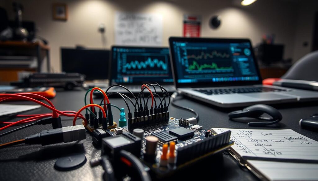
Four magnets on your wheel? Divide by four. This is basic math, but students often forget about sensor setup.
Dewesoft systems support encoder and tachometer inputs for professional speed measurement. But you don’t need expensive equipment to learn the basics. Hall effect sensors offer the same physics at a lower cost.
Pressure averaging requires a bit more thought. Simple arithmetic mean works well for stable processes. But time-weighted averaging is needed when sampling intervals change.
Moving averages smooth out noisy signals. But they reduce the detail of your data. You get clarity but lose some precision.
The Cave Pearl Project teaches simplicity. Start with basic averaging before moving to complex filtering.
Mechanical work estimates dive into thermodynamics. Pressure times volume change equals energy transfer. But you need synchronized pressure and position data, plus chamber geometry knowledge.
For piston engines, indicated mean effective pressure is key. Integrate pressure over volume through the cycle. Then divide by displacement.
This turns raw measurements into useful engineering insights.
| Calculation Type | Formula | Key Requirement | Common Pitfall |
|---|---|---|---|
| RPM from Hall Sensor | (Pulse Count × 60) / (Time × Pulses per Rev) | Known magnet count | Forgetting sensor configuration |
| Arithmetic Mean Pressure | Sum of Values / Number of Samples | Stable sampling rate | Ignoring time intervals |
| Time-Weighted Average | Σ(Value × Duration) / Total Time | Accurate timestamps | Variable interval blindness |
| IMEP Work Estimate | ∫(P dV) / Displacement | Synchronized P-V data | Missing position correlation |
These calculations happen after collecting data, using spreadsheet formulas or Python scripts. You’re turning logged voltages into physical understanding through data processing.
Excel gives quick results—just drag formulas down columns. Python handles bigger datasets well.
Students need to understand that numbers are just the beginning. They’re the raw materials for engineering analysis.
Your Hall sensor counts magnetic transitions, not rpm. You calculate rpm by applying context and configuration knowledge. Your pressure transducer reports voltage proportional to strain, not work.
Without interpretation, measurement is just collecting fancy graphs. Arduino sensors give you data. Understanding requires brain engagement.
Begin with simple rpm calculations. Then, average pressure over ten seconds. Plot results in a spreadsheet to check if they match reality.
Progress to time-weighted averages and work estimates. Each step builds your analytical skills. You learn to see raw sensor output and know what calculations are meaningful.
Dashboard design color coding limits unit conversions
Dashboard design turns raw data into something useful, or it fails and leaves you confused. The difference between a good data logger and a simple number printer is how easy it is to use. If users can’t understand the system status quickly, your design is not effective.
Color coding is not just for looks; it’s based on how our brains work. Green means everything is okay, yellow means pay attention, and red means fix it now. Your RGB LED can show three different colors without needing words.
Make the LED flash green when the BMP280 gets a reading. Use yellow when it’s talking to sensors or moving data. Turn red if the battery gets low or if the readings don’t make sense. This way, complex system states are easy to see.
A good dashboard layout is easy to follow. Put things in order from left to right and top to bottom. Make bigger things more important, not just because they cost more.
Set alert thresholds before things get bad. Show the BMP280 pressure in green if it’s right. Use yellow when it’s getting close to bad. Turn red if it’s impossible, like in a vacuum.
Measurement units can cause trouble in international work. Your sensor uses Pascals because it’s the right unit. But some people might want PSI or millibars. Show both or let users choose, but keep it consistent.
Here’s a table showing how to convert pressure units for student projects:
| Unit Type | Conversion Factor | Typical Use Case | Display Precision |
|---|---|---|---|
| Pascal (Pa) | 1.0 (base unit) | Scientific reporting | ±0.1 Pa |
| Kilopascal (kPa) | 0.001 × Pa | Engineering applications | ±0.01 kPa |
| PSI | 0.000145 × Pa | American tire pressure | ±0.01 PSI |
| Millibar (mbar) | 0.01 × Pa | Meteorology standards | ±0.1 mbar |
The best dashboard answers three questions fast: Is it working? What’s it measuring? Should I be concerned? Don’t add more than that or it gets too complicated.
Visual hierarchy is key, not technical details. A flashing red light gets attention faster than any alarm. Use data visualization like bar graphs and colors to make your dashboard easy to use. If it’s easy to use, people will use it more and make better experiments.
Pitfalls noise ground loops aliasing missing timestamps
Watching your temperature sensor swing wildly between extremes at 60 Hz can be humbling. It shows how Arduino sensors face electrical chaos. Your thermometer might say the room temperature is -40°C to +127°C in seconds.
This isn’t a sensor problem. It’s signal noise, unwanted electrical signals in your data. Imagine trying to talk on a subway with trains passing every 30 seconds.
Ground loops are a classic problem. When you have multiple ground paths, current flows between them. This creates voltage offsets that your Arduino reads as real data.
The math is right, but the measurements are wrong.
To fix this, use star grounding topologies. This means having one ground point for all connections. Sometimes, you need to cut ground traces to make sure there’s only one path. It’s like surgery.
Power supply issues also cause problems. High-current devices like buzzers can mess with your readings. The Cave Pearl Project says this costs students a lot of debugging time.
Decoupling capacitors help by smoothing out voltage changes. They’re used in e360 loggers to handle sudden current spikes without dropping voltage.
Without them, your data logger might think the pressure changed every time it writes to an SD card.
Aliasing artifacts are tricky because they’re mathematically certain. Sampling a 60 Hz signal at 50 Hz will show a 10 Hz oscillation that doesn’t exist. This fake signal is always there in your data.
Nyquist’s theorem is not a suggestion. It’s a mathematical rule. You need to sample at least twice your highest frequency to avoid aliasing.
The data-driven training approach teaches systematic troubleshooting. Aliasing artifacts look real until you understand their math.
Missing timestamps make your data useless. Every reading needs a time stamp. The e360 logger uses a real-time clock for this.
But students often forget to set the clock. This makes their data look like it’s from January 1, 2000. Without time, your data is just numbers.
Debugging hardware teaches you humility. That intermittent connection isn’t a sensor problem. It’s just a breadboard issue. And that weird reading? It’s probably 60 Hz pickup from the lights.
The Cave Pearl Project shows that 15% of parts from cheap suppliers are bad. This isn’t quality control. It’s just the cost of learning electronics.
First-time soldering can damage parts. Forgotten I2C wires and wrong UART settings are common mistakes. These aren’t rare problems. They’re what you learn from.
| Problem Type | Symptom | Root Cause | Solution Strategy |
|---|---|---|---|
| 60 Hz Noise | Oscillating readings at power frequency | Electrical interference from AC power lines | Shielded cables, twisted pairs, physical distance |
| Ground Loops | Voltage offsets, erratic baseline | Multiple ground paths at different potentials | Star grounding topology, single ground reference |
| Power Supply Sag | Readings drop when high-current loads activate | Insufficient supply decoupling | 440µF-1000µF tantalum capacitors near sensors |
| Aliasing Artifacts | False low-frequency signals in data | Sampling below Nyquist frequency | Increase sampling rate, apply anti-aliasing filters |
| Timestamp Errors | Wrong dates, unsorted chronology | RTC not initialized or battery dead | Verify DS3231 settings before deployment |
Building systematic troubleshooting habits is key. Start with power supply checks. Make sure your ground is right. And always check your sampling rates and timestamps.
Remember, component failure is just part of the cost. Ordering extras is smart, not pessimistic. And don’t worry if your soldering doesn’t work at first. It’s just learning.
Data integrity means spotting these problems early. A single 100µF capacitor or a well-set RTC can make all the difference.
The electrical chaos isn’t going away. But you can build systems that can handle it. It’s all about getting the real signal from the noise.
Ethics and safety around data sharing and privacy
Let’s talk about the ethics of data sharing and privacy. Technical skills are important, but ethics are just as critical. That simple temperature logger you’re building? It can become a tool for surveillance in places where people live, work, or gather. It can track who’s there and when.
Every sensor deployment has an ethical side, even if you mean well. A temperature sensor in a classroom can show who’s there. Over time, it can reveal patterns without anyone’s consent. This is the harsh reality of our world filled with sensors.
Privacy matters before you start collecting data, not after. If you’re using sensors in public or shared areas, tell people. Post signs and explain why you’re doing it. Even small data can be used in big ways.
Think about what data can really show:
- How often things are used can reveal schedules and operations
- Temperature data in homes can show who’s there and when
- Door sensors can track who enters and leaves, showing security issues
- Sound levels can tell you how many people are there and when
Information security is key, even for data that seems harmless. A simple file of temperature readings can be very valuable. Treat all data as if it’s sensitive.
Always aim to collect only what you need. Keep data only as long as you have to. Share it only when you have to, and with permission. Delete it when you’re done.
This isn’t being paranoid. It’s about handling data responsibly in today’s world.
Physical safety is just as important as digital ethics. Vaisala systems have special devices for dangerous places. These devices are not just extra safety measures; they’re essential to prevent accidents.
Professional projects need professional safety standards. Sensors in food or medicine need to be sealed to prevent contamination. They must be mounted safely to avoid accidents. And they must be grounded to prevent shocks in wet places.
The Cave Pearl Project shows how to do sensor deployment right. It’s about environmental research with clear goals and minimal privacy impact. But, move that technology to places where people live, and it gets much more complicated. It’s all about the context.
| Deployment Context | Primary Ethical Concern | Privacy Risk Level | Mitigation Strategy |
|---|---|---|---|
| Environmental research outdoors | Data accuracy and scientific integrity | Low | Transparent documentation and data sharing protocols |
| Public indoor spaces | Occupancy tracking without consent | High | Visible signage, aggregate-only reporting, automatic deletion schedules |
| Industrial facilities | Proprietary process exposure | Medium | Secure storage, access controls, non-disclosure agreements |
| Educational laboratories | Student data protection | Medium | Anonymized datasets, clear retention policies, FERPA compliance |
Dewesoft systems are used in critical fields like aerospace and automotive. These industries know that ethics and safety are not limits but must-haves. Your projects should follow these standards too.
Learning to use sensors without thinking about ethics is a problem. You’re not just learning to read thermocouples. You’re learning to use tools that can help or harm, depending on how you use them.
Build sensors that measure what’s important. Use them openly. Handle the data as if it’s someone’s trust. That’s not just idealism. That’s engineering with integrity.
Starter code and CSV template
The Cave Pearl e360 base code is on GitHub, ready for you to explore. It uses the RocketScream LowPower.h library to extend battery life. You can easily add BMP280 pressure sensors by uncommenting a few lines.
Navigation comments labeled STEP1, STEP2, STEP3 are not just for show. They guide you through adding sensors. This is called scaffolding, helping you navigate the code.
For UART connection, use 500,000 baud to access the startup menu. If you get it wrong, you’ll see random characters. The Pro Mini restarts when you close and reopen the serial monitor, fixing display issues.
Your CSV should have timestamp first, followed by sensor headers with units. Use ISO 8601 date format to avoid timestamp confusion. Store sensor outputs as 16-bit integers to keep data clean.
Start with working examples to learn. Changing one thing at a time helps you understand better. This approach makes data formatting more concrete.
